Tuesday, August 29, 2006

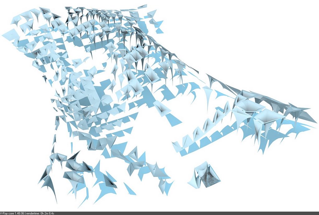
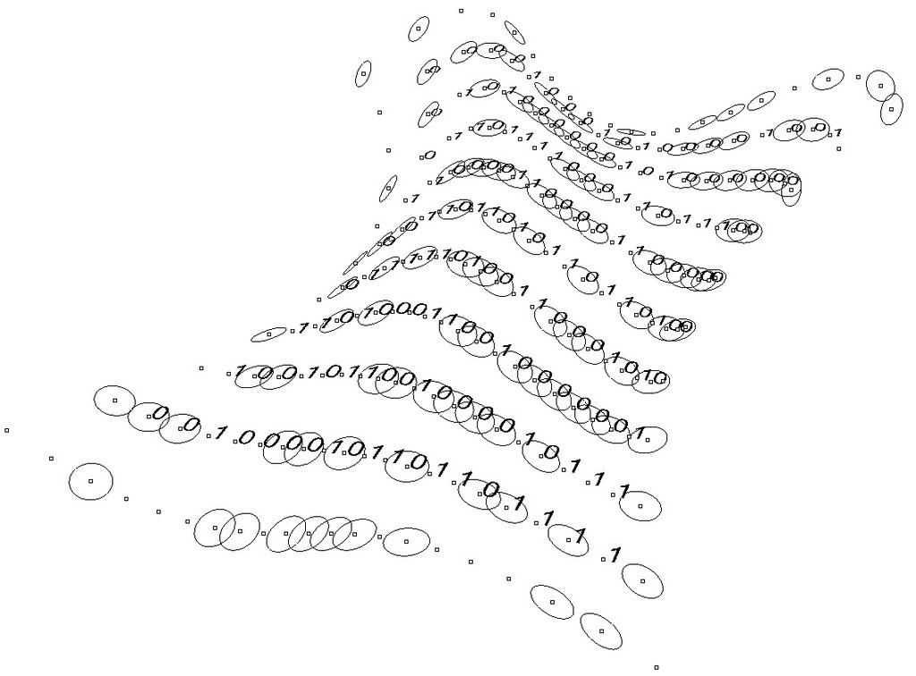
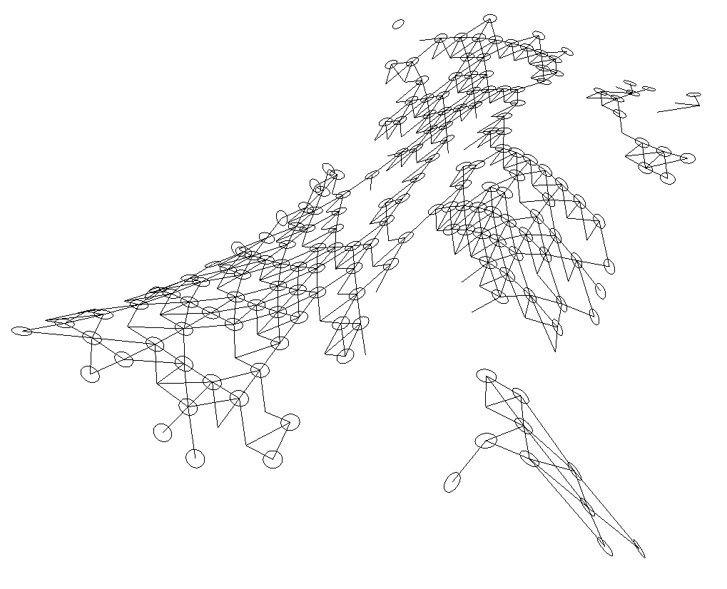
rh4_060829_GameOfLife_RulesAsFunction


' ---------------------------------------------------------------------------------
' Conway's Game of Life
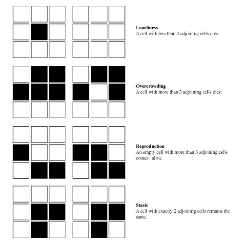
' Rules:
' The universe of the GAME OF LIFE is an infinite two-dimensional grid of cells, each of which Is either alive Or dead.
' Cells interact With their eight neighbours, which are the cells that are directly horizontally, vertically, Or diagonally adjacent.
' At Each Step In Time, the following effects occur:
'
' 1. Any live cell With fewer than two neighbours dies, as If by loneliness.
' 2. Any live cell With more than three neighbours dies, as If by overcrowding.
' 3. Any live cell With two Or three neighbours lives, unchanged, To the Next generation.
' 4. Any dead cell With exactly three neighbours comes To life.
'
' The INITIAL PATTERN constitutes the first generation of the system.
' The Second generation Is created by applying the above rules simultaneously To every cell In the first generation
' -- births And deaths happen simultaneously, And the discrete moment at which this happens Is called a TICK.
' The rules continue To be applied repeatedly To create further generations.
' ---------------------------------------------------------------------------------

' ------------------------------------------------------
' [ CELLULAR AUTOMATON ]
' ------------------------------------------------------
Function newCell(arrCell,i,j)

' Check cell's neigbours
Dim total : total = neighboursCount(arrCell,i,j)
' [ RULES : GAME OF LIFE ]
If (arrCell(i,j) = 1) Then '---------if cell is ON

' LONELINESS: a cell with less than 2 adjoining cells dies
If (total < newcell =" 0"> 3) Then newCell = 0
' STASIS: a cell with exactly 2 adjoining cells remains the same
If (total = 2) Then newCell = 1

Else '---------if cell is OFF

' REPRODUCTION: an empty cell with more than 3 adjoining cells comes alive
If (total >= 3) Then newCell = 1

End If
End Function
' ---------------------------------------------------------------------------------

Friday, August 25, 2006

rh4_060825_Game Of Life


CONWAY'S GAME OF LIFE:

The GAME OF LIFE is a CELLULAR AUTOMATON devised by the British mathematician John Horton Conway in 1970. It is the best-known example of a cellular automaton.

The "game" is actually a ZERO-PLAYER GAME, meaning that its EVOLUTION is determined by its INITIAL STATE, needing no input from human players. One interacts with the Game of Life by creating an initial configuration and OBSERVING how it evolves.


RULES:

The universe of the Game of Life is an infinite two-dimensional grid of cells, each of which is either ALIVE or DEAD. Cells interact with their eight NEIGHBOURS, which are the cells that are directly horizontally, vertically, or diagonally adjacent. At each step in time, the following effects occur:

1. LONELINESS : any live cell with fewer than two neighbours dies.
2. OVERCROWDING : any live cell with more than three neighbours dies.
3. STASIS : any live cell with two or three neighbours lives, unchanged, to the next generation.
4. REPRODUCTION : any dead cell with exactly three neighbours comes to life.

The INITIAL PATTERN constitutes the first generation of the system. The second generation is created by applying the above rules simultaneously to every cell in the first generation -- births and deaths happen simultaneously, and the discrete moment at which this happens is called a TICK. The rules continue to be applied repeatedly to create further generations.


ITERATION:

From an initial pattern of living cells on the grid, observers will find, as the generations tick by, the population constantly undergoing unusual and always unexpected, change. The patterns that form from the simple rules may be considered a form of BEAUTY. In a few cases the society eventually dies out, with all living cells vanishing, although this may not happen until after a great many generations. Most initial patterns either reach stable figures - Conway calls them "still lifes" - that cannot change or patterns that oscillate forever. Patterns with no initial symmetry tend to become symmetrical. Once this happens the symmetry cannot be lost, although it may increase in richness.


ALGORYTHMS:

The earliest results in the Game of Life were obtained without the use of computers. The simplest still-lifes and oscillators were discovered while tracking the fates of various small starting configurations using graph paper, blackboards, physical game boards, for instance Go, and the like. During this early research, Conway discovered that the R-pentomino failed to stabilize in a small number of generations.

These discoveries inspired computer programmers over the world to write programs to track the evolution of Life patterns. Most of the early algorithms were similar. They represented Life patterns as two-dimensional arrays in computer memory. Typically two arrays are used, one to hold the current generation and one in which to calculate its successor. Often 0 and 1 represent dead and live cells, respectively. A double loop considers each element of the current array in turn, counting the live neighbors of each cell to decide whether the corresponding element of the successor array should be 0 or 1. At the end of this process, the contents of the successor array are moved to the current array, the successor array is cleared, and the current array is displayed.

A variety of minor enhancements to this basic scheme are possible, and there are many ways to save unnecessary computation. A cell that did not change at the last time step, and none of whose neighbors changed, is guaranteed not to change at the current time step as well, so a program that keeps track of which areas are active can save time by not updating the inactive zones.

In principle, the LIFE FIELD IS INFINITE, but computers have finite memory, and usually array sizes must be declared in advance. This leads to problems when the active area encroaches on the border of the array. Programmers have used several strategies to address these problems. The simplest strategy is simply to assume that every cell outside the array is dead. This is easy to program, but leads to inaccurate results when the active area crosses the boundary. A more sophisticated trick is to consider the left and right edges of the field to be stitched together, and the top and bottom edges also. The result is that active areas that move across a field edge reappear at the opposite edge. Inaccuracy can still result if the pattern grows too large, but at least there are no pathological edge effects. Techniques of dynamic storage allocation may also be used, creating ever-larger arrays to hold growing patterns. Alternatively, the programmer may abandon the notion of representing the Life field with a 2-dimensional array, and use a different data structure, like a vector of coordinate pairs representing live cells. This approach allows the pattern to move about the field unhindered, as long as the population does not exceed the size of the live-coordinate array. The drawback is that counting live neighbors becomes a search operation, slowing down simulation speed. With more sophisticated data structures this problem can also be largely solved.


technics: first tests on V-Ray for rhino; here Global Illumination with very few settings...

credits: every experiment has its past, future and references... here partly challenged by Chris & Ben (www.terraswarm.com) and some old demons from the AADRl background, theverymany is looking back at "Cellula Automaton" & "A New Kind Of Sciences" from Stephen Wolfram... that is a very Step01...

Labels: , ,

Wednesday, August 23, 2006

Max_060822_On&OnOnComplexity...


COMPLEXITY is the opposite of simplicity ("Wikipedia.org")

Complexity in systems or behaviour is often described as what is "on the EDGE OF CHAOS" - between ORDER and RANDOMNESS... this work - based on particles systems - is a graphical transition with a current research on "Cellular Automata" starting from the "Game of life" rules... (coming!)

Sunday, August 20, 2006

Pshop_060820_manyThoughtsOntoDesignTests...


TEST (or testing)
1. Test and experiment form parts of the scientific method, to verify or falsify an expectation with an observation.
2. Quality control testing, in manufacturing, a procedure designed to test the functionality of a product under potentially harmful conditions

"Be realistic - demand the impossible!" - Soyez réalistes, demandez l'impossible! - Anonymous graffiti, Paris 1968
COLLAGE (From the French, coller, to stick) is regarded as a work of visual arts made from an assemblage of different forms, thus creating a new whole. This technique made its first appearance in the early 20th century as a groundbreaking novelty, however with the passing of time it's become ubiquitous.


DISTINCTION BETWEEN EVALUATION AND ASSESSMENT
In the field of evaluation, there is some degree of disagreement in the distinctions often made between the terms 'evaluation' and 'assessment.' Some practitioners would consider these terms to be interchangeable, while others contend that evaluation is broader than assessment and involves making judgments about the merit or worth of something (an evaluand) or someone (an evaluee). When such a distinction is made, 'assessment' is said to primarily involve characterizations – objective descriptions, while 'evaluation' is said to involve characterizations and appraisals – determinations of merit and/or worth. Merit involves judgments about generalized value. Worth involves judgments about instrumental value. For example, a history and a mathematics teacher may have equal merit in terms of mastery of their respective disciplines, but the math teacher may have greater worth because of the higher demand and lower supply of qualified mathematics teachers. A further degree of complexity is introduced to this argument when working in different languages, where the terms 'evaluation' and 'assessment' may be variously translated, with terms being used that convey differing connotations related to conducting characterizations and appraisals.

"I take my desires for reality because I believe in the reality of my desires" - Anonymous graffiti, Paris, 1968

"Beneath the paving stones - the beach!" - Sous les pavés, la plage! - Anonymous graffiti, Paris 1968

A RESULT is the final consequence of a sequence of actions or events (broadly incidents and accidents) expressed qualitatively or quantitatively, being a loss, injury, disadvantage, advantage, gain, victory or simply a value. There may be a range of possible outcomes associated with an event possibly depending on the point of view, historical distance or relevance.

i.e wikipedia

Sunday, August 13, 2006

Rh4_VoronoiSkeleton..


SELF-SIMILARITY

A SELF-SIMILAR object is exactly or approximately similar to a part of itself, i.e., the whole has the same shape as one or more of the parts. A curve is said to be self-similar if, for every piece of the curve, there is a smaller piece that is similar to it. For instance, a side of the Koch snowflake is self-similar; it can be divided into two halves, each of which is similar to the whole.

Many objects in the real world, such as coastlines, are statistically self-similar: parts of them show the same statistical properties at many scales. Self-similarity is a typical property of fractals.

It also has important consequences for the design of computer networks, as typical network traffic has self-similar properties. For example, in telecommunications traffic engineering, packet switched data traffic patterns seem to be statistically self-similar. This property means that simple models using a Poisson distribution are inaccurate, and networks designed without taking self-similarity into account are likely to function in unexpected ways.

i.e. http://en.wikipedia.org/wiki/Self_similarity

the overall skeleton is an assembly of self-similar cells: those cells are all different but all similar; all the cell's boundaries are the result of the overall split of an host surface based on a VORNOI tesselation algorythm; their geometries have the same genotype: each is created with a developable surface between the exact polyline boundary and its nurbs approximation.


the rhinoscript process is naming and exporting each cell component as a .3ds (thks to David) file which is than open into a PEPEKURA a little origami application (http://www.tamasoft.co.jp/pepakura-en/) which unfold it with laps; an obvious simplifaication of the developable surface has to be done!!!
'------------------------------------------------------
' fileToExportComponents
'Dim Folder, FileName, sPath
''Folder = Rhino.BrowseForFolder(, "Base folder for multi-export", "Multi export")
''FileName = Rhino.StringBox("File name basis", "Export_01", "Multi export")
'------------------------------------------------------
' //////////////////////////////////////////////////////
'' [EXPORT COMPONENTS]
'Rhino.UnselectAllObjects
'Rhino.SelectObjects strLoftSrf
''sPath = Folder & FileName &amp; "_" & i & ".3ds"
'sPath = "E:\RHINOSCRIPTING\060804_Voronoi_M_Corean\060810_Export_Automaton\" & "Export_05" &amp; "_" & i & ".3ds"
'Rhino.Command "-_Export " & Chr(34) & sPath & Chr(34) & " Enter"
'' low mesh
''Rhino.Command "-_Export " & Chr(34) & sPath & Chr(34) & " _DetailOptions _AdvancedOptions _Angle=20 _MaxEdgeLength=3 _Enter _PackTextures=Yes _Refine=Yes _Enter"
' //////////////////////////////////////////////////////

Thursday, August 10, 2006

Rh4_060810_Vorono_2D&1/2


from 2D to "transferOntoSrf"; some sort of 2&1/2D...
' ------------------------------------------------------
' Function transfertPtOntoSrf
Function TransfertPtsOnSrf(arrPt, BBox, targetSrf)
Dim strpolyline, strPlanSrf
Dim tempUVPt
Dim sDomU_PlanSrf, sDomV_PlanSrf
strpolyline = Rhino.AddPolyline(Array(Array(BBox(0)(0)-10, BBox(0)(1)-10, 0), _
Array(BBox(1)(0)+10, BBox(1)(1)-10, 0), _
Array(BBox(2)(0)+10, BBox(2)(1)+10, 0), _
Array(BBox(3)(0)-10, BBox(3)(1)+10, 0), _
Array(BBox(0)(0)-10, BBox(0)(1)-10, 0)))
strPlanSrf = Rhino.addPlanarSrf (Array(strpolyline))
' ------------------------------------------------------
'reparameterize the UV domain of the target surface to match the source surface
sDomU_PlanSrf = Rhino.SurfaceDomain(strPlanSrf(0), 0)
sDomV_PlanSrf = Rhino.SurfaceDomain(strPlanSrf(0), 1)
Rhino.UnselectAllObjects
Rhino.SelectObject targetSrf
Rhino.command("-_Reparameterize " & sDomU_PlanSrf(0) & " " & sDomU_PlanSrf(1) & " " & sDomV_PlanSrf(0) & " " & sDomV_PlanSrf(1) & " ")
' ------------------------------------------------------
tempUVPt = Rhino.SurfaceClosestPoint(strPlanSrf(0), arrPt)
TransfertPtsOnSrf = Rhino.EvaluateSurface(targetSrf, tempUVPt)
' Rhino.addpoint TransfertPtsOnSrf
Rhino.deleteObjects Array(strPolyline,strPlanSrf(0))
End Function
' ------------------------------------------------------

Monday, August 07, 2006

Rh4_060807_VORNOI


In mathematics, a Voronoi diagram, named after Georgy Voronoi, also called a Voronoi tessellation, a Voronoi decomposition, or a Dirichlet tessellation (after Lejeune Dirichlet), is special kind of decomposition of a metric space determined by distances to a specified discrete set of objects in the space, e.g., by a discrete set of points.


DEFINITION
For any (topologically) discrete set S of points in Euclidean space and for almost any point x, there is one point of S closest to x. The word "almost" is occasioned by the fact that a point x may be equally close to two or more points of S.

If S contains only two points, a and b, then the set of all points equidistant from a and b is a hyperplane — an affine subspace of codimension 1. That hyperplane is the boundary between the set of all points closer to a than to b, and the set of all points closer to b than to a. It is the perpendicular bisector of the line segment from a and b.

In general, the set of all points closer to a point c of S than to any other point of S is the interior of a (in some cases unbounded) convex polytope called the Dirichlet domain or Voronoi cell for c. The set of such polytopes tessellates the whole space, and is the Voronoi tessellation corresponding to the set S. If the dimension of the space is only 2, then it is easy to draw pictures of Voronoi tessellations, and in that case they are sometimes called Voronoi diagrams.

The dual for a Voronoi tessellation is the Delaunay triangulation for the same set of points S.


GENERALIZATIONS
Voronoi cells can be defined for metrics other than Euclidean. However in these cases the Voronoi tessellation is not guaranteed to exist (or to be a "true" tessellation), since the equidistant locus for two points may fail to be subspace of codimension 1, even in the 2-dimensional case.

Voronoi cells can also be defined by measuring distances to areas rather than to points. These types of Voronoi cells are used in image segmentation, optical character recognition and other computational applications. In materials science, polycrystalline microstructures in metallic alloys are commonly represented using Voronoi tessellations.
ie WIKIPEDIA


VORNOI CODE (from challenge last week at the office + Rassul...)
The Voronoi core has been developped by David Rutten (reconstructivism.net)

Function VoronoiPolygon(index, datSet, BBox)
' this function creates a voronoi cell for agiven point in a set of points
' should probably be optimized so that it only tests points near the samplepoint
VoronoiPolygon = Null

Dim midPt, arrPt, vecDir(1)
Dim ptS(2), ptE(2)
Dim ChordLength, Border
Dim brdLines(), i, N
ReDim brdLines(UBound(datSet)-1)
ChordLength = Rhino.Distance(BBox(0), BBox(2))

arrPt = datSet(index)
N = 0

For i = 0 To UBound(datSet)
If i <> index Then
midPt = Array((datSet(i)(0) + datSet(index)(0))/2, _
(datSet(i)(1) + datSet(index)(1))/2, _
0)
vecDir(0) = -(datSet(i)(1)-datSet(index)(1))
vecDir(1) = datSet(i)(0)-datSet(index)(0)
vecDir(0) = vecDir(0)/Rhino.Distance(datSet(i), datSet(index))*ChordLength
vecDir(1) = vecDir(1)/Rhino.Distance(datSet(i), datSet(index))*ChordLength
ptS(0) = midPt(0)+vecDir(0)
ptS(1) = midPt(1)+vecDir(1)
ptS(2) = 0
ptE(0) = midPt(0)-vecDir(0)
ptE(1) = midPt(1)-vecDir(1)
ptE(2) = 0
brdLines(N) = Rhino.AddLine(ptS, ptE)
N = N+1
End If

Next

Border = Rhino.AddPolyline(Array(Array(BBox(0)(0)-10, BBox(0)(1)-10, 0), _
Array(BBox(1)(0)+10, BBox(1)(1)-10, 0), _
Array(BBox(2)(0)+10, BBox(2)(1)+10, 0), _
Array(BBox(3)(0)-10, BBox(3)(1)+10, 0), _
Array(BBox(0)(0)-10, BBox(0)(1)-10, 0)))
Rhino.UnselectAllObjects
Rhino.SelectObjects brdLines
Rhino.SelectObject Border
Rhino.Command "-_CurveBoolean _DeleteInput=No _CombineRegions=No " & _
Rhino.Pt2Str(Array(datSet(index)(0),datSet(index)(1),datSet(index)(2))) & _
" _Enter", vbFalse
' delete lines
Rhino.UnselectAllObjects
Rhino.SelectObjects brdLines
Rhino.Command "-_Delete"

VoronoiPolygon = vbTrue
End Function

Labels:

Tuesday, August 01, 2006

Rh4_060801_onTheWayTo_L-Sytems


FROM FRACTALS TO L-SYSTEMS...
going from unifrom growing generation to an alphabet based one...

strCase = Fix(random(2,4))
Select Case CStr(strCase)
Case 2 ...
Case 3 ...
Case 4 ...
End Select

L-SYSTEMS

"The recursive nature of the L-system rules leads to self-similarity and thereby fractal-like forms which are easy to describe with an L-system. Plant models and naturally-looking organic forms are similarly easy to define, as by increasing the recursion level the form slowly 'grows' and becomes more complex.

L-system grammars are very similar to the semi-Thue grammar (see Chomsky hierarchy). L-systems are now commonly known as parametric L systems, defined as a tuple

G = {V, S, ω, P},

where

* V (the alphabet) is a set of symbols containing elements that can be replaced (variables)
* S is a set of symbols containing elements that remain fixed (constants)
* ω (start, axiom or initiator) is a string of symbols from V defining the initial state of the system
* P is a set of rules or productions defining the way variables can be replaced with combinations of constants and other variables. A production consists of two strings - the predecessor and the successor.

The rules of the L-system grammar are applied iteratively starting from the initial state.

An L-system is context-free if each production rule refers only to an individual symbol and not to its neighbours. If a rule depends not only on a single symbol but also on its neighbours, it is termed a context-sensitive L-system.

If there is exactly one production for each symbol, then the L-system is said to be deterministic (a deterministic context-free L-system is popularly called a D0L-system). If there are several, and each is chosen with a certain probability during each iteration, then it is a stochastic L-system.

i.e. Wikipedia